Data

In 3D data visualization, we distinguish two types of 3D data: 3D geometry and data associated with 3D geometry.

• 3D geometry as data: In this category, we are mainly interested in visualizing the shape/location of the 3D geometry. For example, the shape of a deformed mesh or the location of points in a point cloud.
• Data associated with 3D geometry: In this category, the data is a spatially varying field, and we would like to visualize its value at different locations. For example, the Gaussian curvature field on a curved surface, or the geodesic distance on a surface with respect to a source surface point.

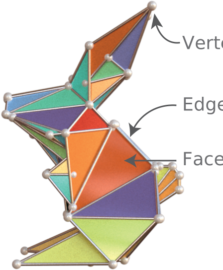
3D geometry are often represented as a mesh for visualization purposes. A mesh, such as the bunny model on the right¹, consists of a set of vertices, edges, and facets. Data associated with 3D geometry are represented as an attribute of a mesh. Each attribute is defined for a specific element type (vertex, edge or facet).

In Hakowan, we leverage Lagrange's SurfaceMesh data structure to represent both 3D geometry and store data associated with 3D geometry as mesh attributes. In a sense, the elements of a mesh defines the "rows" of a 3D data frame, and the attributes of a mesh defines the "columns" of a 3D data frame. In addition, Hakowan can also extract geometry and data associated with geometry from a number of common 3D file formats such as OBJ, PLY, GLTF and MSH.

Hakowan accepts mesh files and Lagrange meshes directly:

l0 = hkw.layer("shape.obj")
l1 = hkw.layer(lagrange.io.load_mesh("shape.obj"))

Numeric arrays with shape (n, 2) or (n, 3) become point clouds. Two-dimensional positions receive a zero Z coordinate:

points = np.array([[0, 0, 0], [1, 0, 0], [0, 1, 0]])
points_layer = hkw.layer(points).mark("point")

Pandas and xarray inputs use x, y, and optional z columns as positions. Use positions= when the columns have domain-specific names. Other numeric columns become vertex attributes, boolean columns are retained as 0/1 attributes, and unsupported non-numeric columns are ignored. Position tables must contain at least one row.

table = pandas.DataFrame({
    "east": [0, 1, 0],
    "north": [0, 0, 1],
    "height": [0, 0, 0],
    "temperature": [12.0, 18.0, 25.0],
})
points_layer = hkw.layer(
    table, positions=("east", "north", "height")
).mark("point")

PyVista polygonal datasets and Trimesh meshes preserve their surface topology, numeric point/vertex attributes, and numeric cell/face attributes:

surface_layer = hkw.layer(pyvista_mesh)
surface_layer = hkw.layer(trimesh_mesh)

These libraries are optional and are not imported by Hakowan. Install all four interoperability dependencies with pip install "hakowan[data]".

Inspecting data

Use hkw.inspect() before building a layer to obtain a JSON-safe summary of the geometry and its attributes. This is useful for scripts and agents that must choose fields without guessing their names or shapes.

summary = hkw.inspect("shape.ply")

print(summary.vertex_count, summary.facet_count)
for attr in summary.attributes:
    print(attr.name, attr.element, attr.channels, attr.minimum, attr.maximum)

# Suitable for JSON serialization or model/tool input.
payload = summary.to_dict()

For indexed attributes, value_count is the number of unique stored values and element_count is the number of indices. Numeric summaries include finite and non-finite row counts, per-channel bounds, and quartiles.

Region of interest

When specifying the data, we can optionally specify a region of interest. The region of interest is an axis-aligned box that defines the region in the center of the rendering.

l0 = hkw.layer().data("shape.obj", roi_box=[[0, 0, 0], [1, 1, 1]])

See the Smoothed Particle Hydrodynamics example for a usage of region of interest.

---

1. 3D model source: origamix rabbit ↩