The Heat Method¶

This example reproduced this figure from the paper "The Heat Method for Distance Computation".

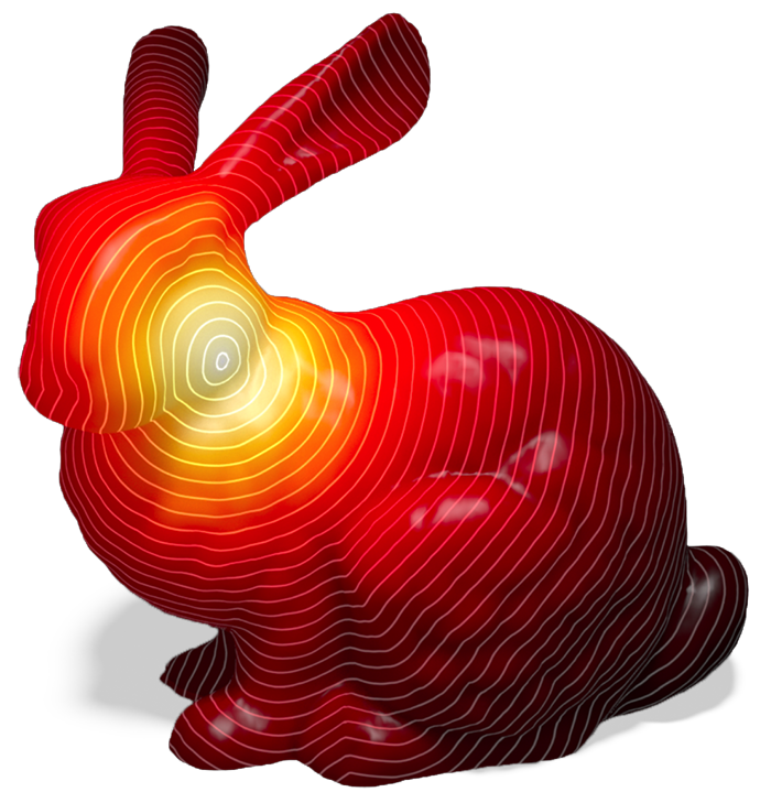
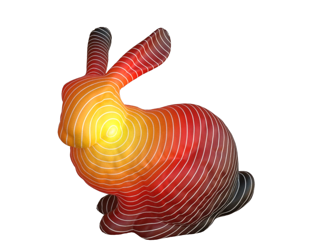
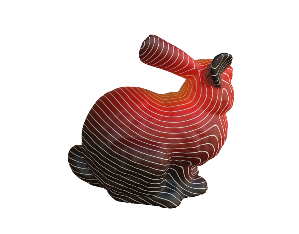
Data¶

The distance field is computed using heat_geodesic method from libigl. The field is stored as dist field in data/bunny_heat.ply.

Input contract¶

mesh: surface from data/bunny_heat.ply; dist (indexed 1-channel scalar).

Reproduce and inspect¶

python ../render_gallery.py --check Heat
python ../render_gallery.py --artifacts Heat

Python · Manifest · Inspection · Canonical JSON · Validation

Code¶

#!/usr/bin/env python

import hakowan as hkw
import math

hkw.set_default_backend("mitsuba")

# Step 1: Create a base layer.
base = hkw.layer("data/bunny_heat.ply").material(
    "Principled",
    # We used isocontour texture to visualize the geodesic distance field both as color
    # and as isocurves.
    color=hkw.texture.Isocontour(
        data="dist",
        texture1=hkw.texture.ScalarField(
            "dist",
            colormap="fire",
            reverse=True,
            domain=(0, 0.12),
            legend=hkw.Legend(title="Geodesic distance"),
        ),
        texture2=hkw.texture.ScalarField(
            "dist",
            colormap=["white", "lightgray"],
            domain=(0, 0.12),
            legend=False,
        ),
        ratio=0.90,
        num_contours=100,
    ),
    roughness=0.5,
)

# Step 2: Declare the shared camera once for every output.
scene = hkw.SceneSettings(
    camera=hkw.PerspectiveCamera(eye=(0, 1.2, 3)),
)
RECIPE_FIGURE = hkw.Figure(base, scene)
RECIPE_INSPECTIONS = {"mesh": "data/bunny_heat.ply"}

# Step 3: Render the image.
hkw.render(RECIPE_FIGURE, filename="results/bunny_heat.webp")

# Step 4: Render the back side.
back_side = base.rotate(axis=[0, 1, 0], angle=math.pi)
hkw.render(hkw.Figure(back_side, scene), filename="results/bunny_heat_back.webp")

# Step 5: Interactive demo
hkw.render(RECIPE_FIGURE, backend="webgl", filename="results/bunny_heat.html")